How to Return Multiple Columns from a Single VLOOKUP in Google Sheets

Do you need to return multiple columns from a single VLOOKUP in Google sheets? If so, you’re in luck! In this blog post, we will show you how to do just that. We will walk you through the example steps, and then give you a few tips on how to make the process even easier. Let’s get started!

What is a VLOOKUP in Google Sheets?

A VLOOKUP, or vertical lookup, is a function in Google sheets that allows you to search for a specific value in a column and return the corresponding data from another column.

Why Would You Want to Use VLOOKUP in Google Sheets?

This is especially useful when you have large sheets of data and need to quickly find specific information. Both advanced and new users will find it satisfying to run the VLOOKUP function and locate a match correctly for what they were looking for.

To use a VLOOKUP, you need to have two columns of data: one with the values you want to search for (the search column), and one with the corresponding data you want to return (the return column).

For example, let’s say you have a sheet of data with customer information, and you want to quickly find the customer’s name and address based on their customer ID. In this case, the customer ID would be the search column, and the name and address would be the return column. There are also some other methods to look up data in Google Sheets, but here we are going to use the VLOOKUP function.

Interesting Read: How to Insert a Check Mark Symbol in Excel

What are the Arguments in VLOOKUP?

VLOOKUP draws on four arguments. They form the basics of carrying out the VLOOKUP function. These include:

1. range_lookup: This argument regulates the type of matching. If it is specified as TRUE, an approximate match will be performed by VLOOKUP. If specified as FALSE, a precise match will be obtained. This argument is set as TRUE by default, so users need to specify if they need an exact match.
2. table_array: This is the range of data in the vertical form the function should “look” through. The first column should contain the lookup variables.
3. lookup_value: The value or element you are searching for
4. column_index_num: This specifies the number of the column where the value is to retrieve it e.g., column 1 is the first column of table_array.

Components of a VLOOKUP Syntax

There are four main components of a VLOOKUP syntax. You can write a normal VLOOKUP function as follows:

                      =VLOOKUP(search_key, range, index, [is_sorted])

In the syntax, search_key is the required value you wish to look up. You can specify the value itself or the cell that holds the value.

The range refers to the cells in your table where VLOOKUP needs to look for the specified search key.

An index is the number of columns holding the required value inside the specified range. Note that the first column within the range has an index of 1, the second column has an index of 2, and so on. Finally, is_sorted refers to the match mode being either TRUE or FALSE. It specifies whether to sort or not sort the search column.

How to Return Multiple Columns from a Single VLOOKUP in Google Sheets

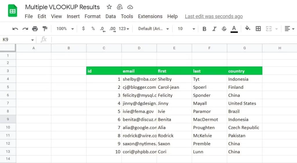
The VLOOKUP function can only look up one column at a time. Also, it is used to look for values in vertical data. This refers to tables like the one shown below. The data must be arranged top to bottom in columns.

You can tweak things a bit to expand it to multiple related columns simultaneously. You can use the ARRAY formula to link more than one field together to use them like multiple criteria within VLOOKUP. This is a standard ARRAY formula syntax:

                           =ARRAYFORMULA(array_formula)

To nest the VLOOKUP function into the ARRAY formula, you can use the following function:

           =ARRAYFORMULA(VLOOKUP(search_key, range, {index}, is_sorted))

Now, let’s get started.

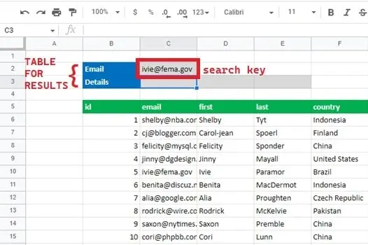
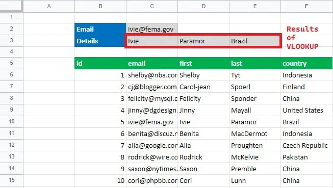
• First of all, make a table where you wish the results of VLOOKUP to display. In this dataset, let us say we want to look up details by mentioning emails. Hence, we make a table with rows titled “Email” in C2 to include the search key, and the cells after “Details” in C3 to display the results after the application of the formula.

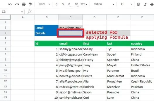
• Click the cell in the spreadsheet where you want to apply the formula and want the result to appear. In this example, cell C3 is selected.

• After selecting the cell, type the following formula in the formula bar and press Enter.

                =ARRAYFORMULA(VLOOKUP(C2,C6:F15,{2,3,4},false))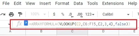

In the formula, we have replaced seaerch_key, range, {index}, is_sorted with our desired values.

• Here, the C2 is the cell holding the search_key. It is the specific cell with the criteria you want to find. In this case, it is an email address. C6:F15 is referring to the range where you want to use the “lookup” technique, which is the range of selected cell numbers you wish to search through. {2,3,4} are the index values i.e., the column numbers in the table of the required value. In our table, Column 2 holds the emails, Column 3 holds the first names, and Column 4 holds the last names. False refers to the range lookup mode, so an exact match is obtained in the results.

• After you press Enter, it will return or retrieve the value in the selected cell. As in the case of our data, the VLOOKUP searched the data by using the email provided as search criteria and displayed the required first name, last name, and country name.

And that’s how you can return multiple columns from a single VLOOKUP in Google sheets. Functions like these are useful to increase productivity and streamline work. No matter where you are at the home, office, or studying, Google sheets functions will make your life easier!

Tips for Using the VLOOKUP Function in Google Sheets

Now that you know how to use the VLOOKUP function in Google sheets, let’s look at a few tips to make the process even easier.

1. Use a Reference Cell for the Search Column

If you are going to be using the VLOOKUP function multiple times, it can be helpful to create a reference cell for the search column. This way, you don’t have to keep typing in the column number each time.

2. Use a Named Range for the Search Column

Another way to make using the VLOOKUP function easier is to use a named range for the search column. A named range is simply a way of giving a cell or range of cells a name. This can be especially helpful if the column you are searching for is not in the first column of your data. To create a named range, select the cells you want to include in the range, and then click Data > Named ranges. Enter a name for the range, and then click OK.

3. Use the Wildcard Character (*) in the Search Value

If you are not sure of the exact value you are looking for in the search column, you can use the wildcard character (*) to return all values that contain a certain string of characters.

4. Use the IFERROR Function to Handle Errors

If you’re using the VLOOKUP function on a large sheet of data, there’s a chance that an error will occur if the value you’re looking for isn’t in the search column. To avoid this, you can use the IFERROR function to return a blank cell or a custom message.

5. Use the ARRAYFORMULA Function to Return Multiple Columns

If you want to return multiple columns from a single VLOOKUP, you can use the ARRAYFORMULA function. This function allows you to enter an array of formulas and return the results as a single array.

Using VLOOKUP Function in Google Sheets

The VLOOKUP function is a powerful tool for finding data in Google sheets. By understanding the arguments and how to return multiple columns from a single VLOOKUP, you can use this function to quickly and easily find the data you need. Have you tried using the VLOOKUP function in your own Google sheets? What tips do you have for making this function work for you?

Note: Does this article provide the info you’re looking for? Is there any information you think of missing or incorrect? You can give your opinion in the comments section below.

If you like this tutorial, share this post and spread the knowledge by clicking on the social media options below because “Sharing is caring”